Towards a holistic formalization of ETH
The derivations below are highly preliminary and incomplete. There are plenty of things that need to be accounted for and fixed. See Issues/Ideas. Comments are welcome.
Here’s a presentation I made to the research team at the Ethereum Foundation and Columbia’s CryptoEconomics Conference: here
1.1 Valuation equation
Assuming all new issuance and fees accrue to existing ETH holders, we can express the valuation of ETHUSD $M^\ast_{t}$ at time $t$ as:
\[M^\ast_{t}=p^\ast_{t}S_t=\frac{\bigg(\overbrace{F^{\$}}^{\text{fees/mev}}+\overbrace{\frac{\theta_tA_t^{\$}\pi_t}{1+\pi_t}}^{\text{seigniorage}}\bigg)(1+g_{A^{\$}})}{r_d-g_{A^{\$}}}+\overbrace{\theta_tA_t^{\$}}^{\text{convenience}} \tag{1}\]where $p^\ast_{t}$ is the fundamental ETHUSD rate at time $t$, $S_t$ is the supply of ETH, $F_{t}^{\$}$ is the total USD value of gas fees, $g_{F^{\$}}$ is the growth rate in the USD value of fees $p_tF_t$ and $r_d$ is the discount rate which can also be expressed as $r_f+r_p$ where $r_f$ is the risk-free rate and $r_p$ is a risk premium from a standard capital asset pricing model:
\[r_p=\beta_a[E(r_a)-r_f]\tag{2}\]where $E(r_a)$ is the expected return on some risk factor $a$ and $\beta_a$ is calculated as:
\[\beta_a=\frac{\rho_{e,a}\sigma_e}{\sigma_a} \tag{3}\]where $\rho_{a,m}$ is the correlation between the returns of ETHUSD and $a$, $\sigma_e$ is the volatility of the ETHUSD rate, and $\sigma_a$ is the volatility of the benchmark. In practice, $(2)$ would have more than one factor:
\[r_p=\beta_0[E(r_0)-r_f]+\beta_1[E(r_1)-r_f] \ldots + \beta_n[E(r_n)-r_f]\tag{4}\]Above is a pricing model based on traded factors. However, risk factors need not be directly traded. Expected returns can be estimated via a two-step regression a la Chen, Roll, and Ross (1986). The rightmost terms of $(1)$ is the USD value of ETH convenience holdings, which we denote $H^{\$}$, where $A_t^{\$}$ is the amount $F_t^{\$}+N_t^{\$}$ where $N_t^{\$}$ is the total USD value of ETH denominated consumption excluding gas fees from $t$ to $t+1$ and $\theta_t\in[0,1]$ is a constant and is determined according to a money demand function:
\[\theta_tA^{\$} = -\tau E(\pi_t)\]where $\tau$ is a constant, $E(\pi_t)$ is the expected rate of inflation which we define as the expected percentage change in the outstanding supply of ETH. Also, seigniorage contains two components: an inflation tax and the change in users convenience holdings. So, we can express it as:
\[\frac{\theta_tA_t^{\$}\pi}{1+\pi}(1+g_{A^{\$}})=\underbrace{\theta_{t}A_{t}^{\$}(1+g_{A^{\$}})-\theta_{t}A_{t}^{\$}}_{\text{change in convenience holdings}}-\underbrace{\frac{g_{A^{\$}}-\pi}{1+\pi}\theta_{t}A_{t}^{\$}}_{\text{inflation tax}}\]The inflation tax is a transfer of market capitalization from non-stakers to stakers whereas the latter increases the total market capitalization of ETH.
1.2 Non-reflexive assumption
An important assumption we are making is that $F^{\$}$ is independent of $p$. Proceeding with logarithms denoted by dots, consider:
\[\dot{F}^{\$} =\dot{\mu}^{\$}+\dot{G} \tag{5}\]where $\dot{\mu}^{\$}$ is the log weighted average gas price in USD and $\dot{G}$ is the log amount of gas consumed. Expressing $\dot{F}^{\$}$ as a function of $\dot{p}$ and other exogenous variables:
\(\dot{F}^{\$} = \alpha_{}+ \beta_{\dot{p}}\dot{p}+ \sum_{v=0}^n{\beta_{v}\dot{x}_{v}} \tag{6}\) where $\dot{x}_v$ is the logarithmic value of the $v$th variable. Equivalently, $(6)$ can be rewritten as:
\[\dot{F}_{t} = (\alpha_{\dot{p},\dot{\mu}^{\$}}+ \alpha_{\dot{p},\dot{G}})+(\beta_{\dot{p},\dot{\mu}^{\$}}+ \beta_{\dot{p},\dot{G}})\dot{p}_t + \sum_{v=0}^n{(\beta_{v,\dot{\mu}}+\beta_{v,\dot{G}})\dot{x}_{v}} \tag{7}\]where $\alpha_{\dot{\mu}^{\$}},\beta_{\dot{\mu}^{\$}},$ and $\alpha_{\dot{G}},\beta_{\dot{G}}$ are the coefficients from performing $(6)$ on $\dot{\mu}^{\$}$ and $\dot{G}$ individually instead of on $\dot{F}^{\$}$. Since we are assuming that $\dot{F}^{\$}$ is independent of $\dot{p}$, it should be true that:
\[\beta_{\dot{p},\dot{\mu}^{\$}}+\beta_{\dot{p}, \dot{G}}={0} \tag{8}\]A simple experiment testing the veracity of this assumption can be found in the Appendix.
1.3 Actors
From our valuation equation, we can say that the leftmost term is held by investors and the convenience term is held by users:
\[\underbrace{\frac{\bigg(F^{\$}+\frac{\theta_tA_t^{\$}\pi_t}{1+\pi_t}\bigg)(1+g_{A^{\$}})}{r_d-g_{A^{\$}}}}_{\text{investors}} +\underbrace{\theta_tA_t^{\$}}_{\text{users}} \tag{1}\]1.4 Gas fee mechanism
Under EIP-1559, total ETH fees are the sum of two components: base and priority fees. The base fee price in ETH is calculated as:
\[f^b_t=\bigg[1 + \frac{1}{8} \bigg(\frac{G_{t-1}-G^\ast}{G^\ast}\bigg)\bigg]f^b_{t-1} \tag{9}\]where $G_t$ is the amount of gas used which is currently set to a maximum of 30 million, $G^\ast$ is the target amount of gas per block currently set to 15 million. The priority gas price $f^p_{t}$ is equal to:
\[f^p_t=f_t-f^b_t \tag{10}\]where $f_t$ is the total ETH gas price. Therefore, the USD amount of fees paid is equal to:
\[p_tF_t=p_tG_tf_t=p_tG_t(f^p_t+f^b_t) \tag{11}\]The base fees, $F^b_t=G_tf^b_t$, are burnt and priority fees, $F^p_t=G_tf^p_t$, go directly to validators.
1.5 Issuance
For algorithmically determined issuance, we can place a mechanism on a spectrum between a fixed reward rate $kS^s$, where $k$ is a scalar and $S^s$ is the amount of ETH staked which is equal to $S\lambda$ where $\lambda$ is the staking ratio, and a fixed total reward $k \frac{S^s_i}{\sum_{j=1}^n{S^s_j}}$. We can express the percentage yield earned by stakers $\hat{i}_t$ as:
\[\hat{i}_t=\frac{k}{(S^s_t)^x} \tag{12}\]and total ETH issuance as:
\[i_t=k(S^s_t)^{1-x} \tag{13}\]When $x$ is equal to 1, the amount issued is constant. When $x$ is equal to 0, the yield is constant. Therefore, the smaller $x$ is, the yield and staking ratio are less and more volatile, respectively. Ethereum has chosen a middle ground between fixed rate and fixed total reward. The maximum annual amount of ETH issued $i_{t}$ is determined by:
\[i_t=166.4(S^s_t)^{\frac{1}{2}} \tag{14}\]The $166.4$ is equal to $2.6 \times 64$ where $64$ is the base reward factor and $2.6 \approx \frac{82181.25}{\sqrt{10^9}}$ where $82181.25$ is the number of epochs per year. ETH issuance increases with the amount staked but at a decreasing rate.
1.6 Reinvestment and variance
However, there is randomness in the selection of duties which pay different rewards and those with larger stakes are able to reinvest more quickly in new validators, creating a wedge between the expected and realized yield which is dependent on the size of an individual’s total stake. The annual realized compounded issuance yield (rename capital accumulation rate?) for ETH, $i^*$, is equal to:
\[i^*=\bigg(1+\frac{\hat{i}}{\gamma}\bigg)^{\gamma}-1 \tag{15}\]where $\gamma$ is the reinvestment rate per year. The reinvestment rate $\gamma$ for an individual staking $\bar{S}^s$ ETH is equal to:
\[\gamma=\frac{\bar{S}^{s}\hat{i}}{\phi} \tag{16}\]where $\bar{S}^s$ is the total amount of ETH staked by said individual and $\phi$ is the minimum amount of ETH to launch a new validator which is currently 32 ETH. If you are in a stake pool $z$, $\bar{S}^s$ is the amount staked in the pool and each participant reinvests at $\gamma_{z}$. The expected yield from issuance for a solo validator is equal to:
\[\hat{i}=\varphi(\hat{i}_p)+(1-\varphi)(\hat{i}_a)=(\hat{i}_p-\hat{i}_a)\varphi+\hat{i}_a \tag{17}\]where $\hat{i}_p$ is the yield for being chosen as a block proposer, $\hat{i}_a$ is the yield for attesting to block, and $\varphi$ is $\frac{32}{S^s}$. The proposal and attesting yields can also be expressed as:
\[\hat{i}_p=\frac{i\xi}{\phi}, \hat{i}_a=\frac{i(1-\xi)}{S^s-\phi} \tag{18}\]where $\xi$ is a fixed parameter between 0 and 1 allocating total ETH rewards between proposing and attesting. Currently, the value $\xi$ is set to $\frac{1}{8}$. The variance $\sigma^2$ is equal to:
\[\sigma^2=E(\hat{i}^2)-E(\hat{i})^2 \tag{19}\]where $E(\hat{i}^2)$ is:
\[E(\hat{i}^2)=\varphi(\hat{i}_p)^2+(1-\varphi)(\hat{i}_a)^2 \tag{20}\]$E(\hat{i})^2$ is:
\[E(\hat{i})^2=((\hat{i}_p-\hat{i}_a)\varphi+\hat{i}_a)^2 \tag{21}\]Therefore:
\[\sigma^2=\big((\hat{i}_p^2-\hat{i}_a^2)\varphi+\hat{i}_a^2\big)-((\hat{i}_p-\hat{i}_a)\varphi+\hat{i}_a)^2 \tag{22}\]If $y$ has multiple validators, the variance scales by $\frac{1}{(V^y)^2}$ where $V^y$ is the number of validators controlled by $y$ or by the pool that $y$ is in. The standard deviation of returns is simply the square root of the variance which scales linearly by the number of validators controlled $\frac{1}{V^y}$. In other words, smaller total stakes result in higher variance. The standard deviation $\sigma$ is simply $\sqrt{\sigma^2}$. Therefore, the risk adjusted yield would be $\frac{\hat{i}}{\sigma \Lambda}$ where $\Lambda$ is an annualization factor, if needed.
1.7 Investor objective function
With an investable set $(\text{solo}, \text{lend}, \text{pool}1, \dots\ \text{, pool}{\text{N}})$ we can express it as:
\[\begin{equation} \begin{aligned} \max_{w} \quad & w^T\mu-\frac{\lambda}{2}w^T\Sigma w \\ \text{s.t.} \quad & \textbf{1}^Tw=1 \\ \quad & 0\le w \\ \quad & w_{\text{solo}}=0 \quad \text{if } w_{\text{solo}}S^y < \phi \\ \quad & \bigg(\sum_{i=1}^N{w_{\text{pool}_i}d_i}\bigg)\ell_{\text{pool}} \ge d_{\text{target}} \quad \text{if } \bigg(\sum_{i=1}^N{w_{\text{pool}_i}}\bigg) > 0 \end{aligned} \end{equation}\]where $w$ is a vector of weights, $\mu$ is a vector of returns, $\lambda$ is a risk aversion parameter, $d_i$ is a “decentralization” score of pool $i$, $\ell_{\text{pool}}$ scales the sum of weights across pools to 1, and $\Sigma$ is a covariance matrix. All pools are liquid staking pools and thus have a token. The expected return to solo staking is $\mu_{\text{solo}}-c$, where $c$ is the dollar cost and complexity of running validators which is only available if the allocation is greater than or equal to the minimum amount to solo stake $m_{eb}$. The expected return of a liquid staking pool is:
\[\mu_{\text{pool}}=\mu_{p}-\mu_d+\mu_r(1-f)-\mu_s\]where $\mu_p$ is the expected price return, $\mu_d$ the expected price discount relative to ETH, $\mu_r$ the expected reward rate, $f$ is the fee percentage, and $\mu_s$ is the expected slippage from trading the liquid staking token. The variance of returns from staking in a liquid staking pool are:
\[\sigma^2_{\text{pool}}=\sigma^2_p+\sigma^2_r+\sigma^2_s\]We can think of lending returns and variance analogously (e.g. aTokens on Aave).
For solo validator operators and pools, if we (wrongly) assume for now that all node types are equally as reliable and costless, build a maximum decorrelation portfolio of nodes:
\[\begin{equation} \begin{aligned} \min_{w} \quad & w^TCw \\ \text{s.t.} \quad & \textbf{1}^Tw=1 \\ \quad & w=0 \quad \text{or} \quad w_{-} \le w \le w_{+} \\ \end{aligned} \end{equation}\]where $w, w_-, w_+$ are vectors of weights, minimum required amount of ETH to run a validator, and maximum effective balance, respectively and $C$ is a correlation matrix of node characteristics. Once you have $w$, maximize number of validators on each node since they are imperfectly correlated and virtually costless.
1.8 Staking ratio
From our valuation equation $(1)$ the proportion of ETH not staked or lent is equal to:
\[I= \theta_t\frac{A_t^{\$}}{M^\ast_t} \tag{23}\]Therefore, the staking ratio is $(1-\theta_t\frac{A_t^{$}}{M^\ast_t})(1-w_{\text{lend}})$. Note, we need to consider returns to staking net of fees if we are considering liquid staking.
1.9 Burn rate
The expected burn rate $\Omega$ is equal to:
\(\Omega=\frac{F^{b,\$}_t}{M^\ast_t} \tag{25}\)
2.0 Inflation
We can calculate the implied rate of inflation which, again, we define as the percentage change in the outstanding supply of ETH. The rate of issuance $i^\prime$ is equal to the deposit ratio $\lambda$ times the yield earned by stakers $\hat{i}$:
\[i^\prime=\lambda\hat{i} \tag{26}\]The deposit ratio is equal to $\frac{S^s}{S}$. Therefore, the expected rate of inflation $\pi$ is:
\[\pi=\lambda\hat{i}-\Omega \tag{27}\]The rate of inflation is equal to the deposit rate times the staking yield minus the burn rate.
2.1 ETH/stETH rate
With an amount $\bar{S}^{s}_{t}$ of ETH staked in a liquid staking protocol and amount of $\ddot{S}_t$ derivative tokens in circulation, the price $\ddot{p}$ should be no more than:
\[\ddot{p}_t=\frac{\bar{S}^{s}_{t}}{\ddot{S}_t} \tag{28}\]However, there is a delay in redemption. User $y$ needs to redeem $\ddot{S}^y_t$ stETH tokens for ETH at time $t$ which in excess of the amount in the protocol buffer $b_t$ amounts to $\bar{S}^{s,y}_{t}$ ETH:
\[\bar{S}^{s,y}_{t}=\ddot{S}^y_t\ddot{p}_t-b_t \tag{29}\]We assume the buffer processes withdrawals first-come-first-served. For user $y$ to instantly redeem, she needs to take out a loan of $\phi_t$ ETH with a collateral ratio of $\frac{\bar{S}^{s}_{t}}{\ddot{S}_t}$ for duration $T$ which is the amount of time it takes to unstake from the liquid staking protocol at an interest rate $\zeta_t$:
\[\phi_t(1+\zeta_t)^T=\bar{S}^{s,y}_{t} \tag{30}\]If we set $\bar{S}_{t}^{s,y}$ to $\bar{S_t}^{s}$ this means the price is no less than:
\[\ddot{p}_t=\frac{\phi_t-\kappa}{\ddot{S}_t} \tag{31}\]where $\kappa$ is the ETH transaction cost to repay the loan since we assume that the costs to sell the liquid staking token and initiate the loan are the same. The variation between the bounds is determined by the demand for converting staked ETH into ETH, the time it takes to unstake from Ethereum, the amount in the liquid staking protocol buffer, and the willingness of ETH holders to lend to staked ETH holders.
The amount of time $T$ is determined by the amount of time to unstake and the accumulated amount of unstaked ETH in the protocol. To be clear here, regardless of $T$ below, the $T$ above takes into account the amount of time it takes to withdraw over some period of time using the protocol buffer, e.g. can withdraw from the buffer over a few days instead of having to directly withdraw from Ethereum.
A full withdrawal directly from Ethereum is when you want to full exit the network voluntarily with 32 or less ETH. When you want to perform a full withdrawal you must sign a message that you would like to exit which places you in the exit queue. The total number of validators that can perform a full withdrawal each epoch $V^f$ is determined by:
\[V^f = \max \left(4, \left\lfloor\frac{V}{65536}\right\rfloor\right) \tag{32}\]where $V$ is the total number of validators. Once in the exit queue, the amount of days it takes to reach the exit epoch, when your stake is no longer earning rewards or subject to slashing, is equal to:
\[T^x=\max\bigg(.0178, \frac{V^x}{V^f\epsilon}\bigg) \tag{33}\]where $\epsilon$ is the number of epochs per day and is currently equal to $225$, $V^x$ is the number of full withdrawals in the exit queue, and $.0178$ corresponds to the minimum number of epochs needed to be in the exit queue, currently $4$, which is $25.6$ minutes, or $\approx .0178$ days. Then, the amount of time from the exit epoch to the withdrawal epoch $T^e$ is $256$ epochs, or $\frac{256}{\epsilon} \approx 1.4$ days. Once in the withdrawal epoch, a full withdrawal needs to wait for its turn in a validator sweep. A validator sweep cycles through each validator in order of validator ID and checks if they are eligible for a partial or full withdrawal. A partial withdrawal is any amount of ETH in excess of 32 ETH. Each block can process up to 16 withdrawals, partial or full. The number of blocks per day $B$ is equal to:
\[B=\frac{24 \times 60 \times 60}{T^B}-m \tag{34}\]where $T^B$ is amount of time in seconds for a single block which is currently 12 seconds and $m$ is the number of missed blocks per day. The first term is the number of slots per day. Which means the number of withdrawals per day is equal to $W=16B$. The amount of days in the withdrawal queue is equal to:
\[T^w=\frac{V^x+V^w+V^{p}}{W} \tag{35}\]Therefore, the total time to withdraw directly from Ethereum $T_d$ is equal to:
\[T_d=T^x+T^e+T^w \tag{36}\]It does not cost any ETH for full or partial withdrawals and it is not possible to withdraw any specific amount.
We also need to consider the the expected buffer inflows since we already consider the amount currently in the buffer $b_t$. The number of days to unstake from the liquid staking protocol $T_l$ utilizing only the buffer is:
\[T_l=\frac{\ddot{S}^y_t\ddot{p}_t-b_t}{\Delta_b} \tag{29}\]where $\Delta_b$ is the expected average daily inflow into the buffer. If a staker decides to utilize future buffer flows she can pay off the principal over the life of the loan thus reducing interest expenses.
2.2 Expected returns
The change in market capitalization from $t$ to $t+1$ is equal to:
\[E(r^M_{t,t+1})=g_{A^{\S}} \tag{37}\]The expected return earned by a staker from $t$ to $t+1$ is equal to:
\[E(r^s_{t,t+1})=\widehat{F}^p_{t,t+1}+\hat{i}_t+\frac{g_{A^\$}-\pi_{t,t+1}}{1+\pi_{t,t+1}} \tag{37}\]where $\widehat{F}^p_{t,t+1}$ is the priority fee yield equal to $\frac{F^p_{t+1}p_{t+1}}{S^s_tp_{t}}$. The expected return earned by a non-staker, or the percentage change in $p_t$, from $t$ to $t+1$ is equal to:
\[E(r^u_{t,t+1})=\frac{g_{A^{\$}}-\pi_{t,t+1}}{1+\pi_{t,t+1}} \tag{38}\]The difference in expected return between staked and unstaked ETH is:
\[E(r^s_{t,t+1})-E(r^u_{t,t+1})= \widehat{F}^p_{t,t+1}+\hat{i}_t \tag{39}\]2.3 Value transfer
In each block, ETH holders $\eta$ swap their ETH for blockspace and those who do not $\gamma$. If the ETHUSD rate is overvalued, it is a transfer of value from $\gamma$ to $\eta$. Formally, the amount of value transferred from $\gamma$ to $\eta$ is:
\[M^\ast_{\eta,t}-M^\ast_{\gamma,t}=p_tF_{\eta,t}\bigg(1-\frac{p^\ast_t}{p_t}\bigg) \tag{40}\]Thus, valuation bubbles could serve as a deterrent to staking.
2.4 Objective function
An oversimplified objective function can take the form:
\[\max \quad f(\text{market capitalization, staking ratio, distribution, censorship cost})\]The minimum USD cost to attack Ethereum $\Psi$ is equal to:
\[\Psi_t = \frac{1}{3}M_t\lambda_t \tag{41}\]If a single entity or multiple colluding entities control, or have the ability to control, more than $\Psi$ worth of ETH, they can disrupt Ethereum’s security. Thus, an objective function for the design of the ETH token can be:
\[\max_{} \quad f(\Psi_t, \hat{\Phi}_t) \tag{42}\]where $\Phi$ is some measure of “decentralization.” For simplicity, we use a modified version of the Nakamoto coefficient of ETH ownership. Given there are $H$ entities that hold ETH and the USD value of staked $\varrho_i^s$ and unstaked $\varrho^u_i$ ETH held by entity $i$ where $\sum_{i=1}^H \varrho_i^s + \sum_{i=1}^H \varrho_i^u=M_t$, the Nakamoto coefficient is:
\[\Phi = \min{} \bigg\{ {h\in[1,\dots,H]}:\sum_{i=1}^{h}{\varrho^s_i+\frac{\Psi\varrho^u_i}{\Psi+\varrho^u_i} \geq \Psi} \bigg\} \tag{43}\]In words, the Nakamoto coefficient is the minimum number of entities needed to be colluded to disrupt the network. Need to clarify this logic: the augmentation of the unstaked ETH reflects that it is cheaper to purchase staked ETH, unstake it, and restake it in your own validator relative to purchasing unstaked ETH and then staking it. With liquid staking tokens, we can express $(43)$ as:
\[\Phi = \min{} \bigg\{ {h\in[1,\dots,H]}:\sum_{i=1}^{h}{\varrho^s_i+\varrho^{u,l}_i+\frac{\Psi\varrho^{u,e}_i}{\Psi+\varrho^{u,e}_i} \geq \Psi} \bigg\} \tag{44}\]where $\varrho^{u,l}$ is the USD amount of ETH that can be redeemed from liquid staking pools and $\varrho^{u,e}$ is the amount of unstaked tokens in excess of $\varrho^{u,l}$, thus $\varrho^u=\varrho^{u,l}+\varrho^{u,e}$.
On its own, $(44)$ fails to take into account the independence of each entity. Therefore, the Nakamoto coefficient is applied across multiple dimensions which can span social, political, and economic variables. For example, if entities were grouped by country $c \in{[1,\dots,C]}$ where $C$ is the number of countries represented, equation $(44)$ would become:
\[\Phi = \min{} \bigg\{ {c\in[1,\dots,C]}:\sum_{i=1}^{c}{\varrho^s_i+\varrho^{u,l}_i+\frac{\Psi\varrho^{u,e}_i}{\Psi+\varrho^{u,e}_i} \geq \Psi} \bigg\} \tag{45}\]where $\varrho^s_i$ and $\varrho_i^u$ are the total USD amounts of staked and unstaked ETH held in country $i$. We apply equation $(44)$ across $D$ dimensions and take the minimum value:
\[\hat{\Phi} = \min{} \{\Phi_1,...,\Phi_D\} \tag{45}\]This value somehow needs to be comparable to the profit to attack.
2.5 Accounting
2.5.1 One period, solo participants
2.5.1.1 Accounting
Imagine there are only three individuals in the Ethereum ecosystem with permanent roles: a staker, a buyer, and a seller. The total supply of ETH $S_t$ at time $t$ is:
\[S_tp_t=\big(S^{s}_t+S^b_t+S^l\big)p_t\]where $S^s, S^b, S^l$ is the supply of ETH held by the staker, buyer, and seller, respectively and $p$ is the ETHUSD rate. The staking ratio $\theta$ is thus:
\[\theta_t=\frac{S^s_t}{S_t}\]Assuming instantaneous receipt and restaking of rewards and priority fees and no MEV, the supply of ETH held by the staker in the next period $S^{s}_{t+1}$ is:
\[S^{s}_{t+1}p_{t+1}=\big(S^{s}_t+k\big(S^s_t\big)^{1-x}+f^{p}_tG_t\big)p_{t+1}\]where $k$ and $x$ are constants, $f^{p}$ is the priority fee per unit gas, and $G$ is the total amount of gas used. The term $k\big(S^s_t\big)^{1-x}$ is the reward of newly issued ETH to stakers for following the protocol’s rules. The staking ratio at $t+1$ is:
\[\theta_{t+1}=\frac{S^s_{t+1}}{S_{t+1}}\]Assuming gas fees are not subsidized by sellers, the supply of ETH held by the buyer at $t+1$ is:
\[S^{b}_{t+1}p_{t+1}=\big(S^{b}_t-A_t-(f^b_t+f^{p}_t)G_t\big)p_{t+1}\]where $A$ is the amount of ETH to be transferred to the seller in a single transaction for some ETH denominated service and $f^b$ is the base fee per unit gas. The amount $f^bG$ is burned by the protocol. The supply of ETH held by the seller at $t+1$ is thus:
\[S^{l}_{t+1}p_{t+1}=\big(S^{l}_t+A_t\big)p_{t+1}\]The ETHUSD rate at $t+1$ is:
\[p_{t+1}=p_t(1+\delta_{t,t+1})\]where $\delta_{t,t+1}$ is the percentage change in the ETHUSD rate from $t$ to $t+1$ and is calculated as:
\[\delta_{t,t+1}=\frac{-\pi_{t,t+1}}{1+\pi_{t,t+1}}\]where $\pi_{t,t+1}$ is the percentage change in the ETH supply. The supply of ETH from $t$ to $t+1$ evolves as:
\[S_{t+1}=S_t+k\big(S^s_t\big)^{1-x}-f^b_tG_t\]Therefore, $\pi_{t,t+1}$ is equal to:
\[\pi_{t,t+1}=\frac{k\big(S^s_t\big)^{1-x}-f^b_tG_t}{S_t}\]2.5.1.2 USD financial returns
We formalize the USD financial returns for each of the three individuals. The return for the staker $r^s_{t+1}$ is
\[r^s_{t+1}= \frac{S^s_tp_{t+1}-S^s_tp_t}{S^s_tp_t}+\frac{f^{p}_tG_tp_{t+1}}{S^s_tp_t}+\frac{k\big(S^s_t\big)^{1-x}p_{t+1}}{S_tp_t}\]The first term is the change in USD value of the staker’s existing holdings, the second term is the priority fee yield, and the last term is the reward yield. Equivalently, inserting the equation for the percentage change in the price $\delta_{t,t+1}$ and simplifying, we can express it as:
\[r^s_{t+1}= \frac{\bigg(f^{p}_tG_t+k\big(S^s_t\big)^{1-x}\bigg)}{S^s_t}(1+\delta_{t,t+1})+\delta_{t,t+1}\]The return for the buyer $r^b_{t+1}$ is:
\[r^b_{t+1}=\frac{\big(S^{b}_t-A_t-(f^b_t+f^{p}_t)G_t\big)p_{t+1}}{S^b_tp_t}=\frac{\big(S^{b}_t-A_t-(f^b_t+f^{p}_t)G_t\big)}{S^b_t}(1+\delta_{t,t+1})+\delta_{t,t+1}\]The return for the seller $r^l_{t+1}$ is:
\[r^l_{t+1}=\frac{\big(S^{l}_t+A_t\big)p_{t+1}}{S^l_tp_t}=\frac{\big(S^{l}_t+A_t\big)}{S^l_t}(1+\delta_{t,t+1})+\delta_{t,t+1}\]2.5.2 One period, multiple participants
2.5.2.1 Accounting
Imagine there are many individuals in the Ethereum ecosystem with permanent roles: stakers, buyers, and sellers. The total supply of ETH $S_t$ at time $t$ is:
\[S_tp_t=\big(S^{s}_t+S^b_t+S^l\big)p_t\]where $p$ is the ETHUSD rate and $S^s, S^b, S^l$ is the supply of ETH held by stakers, buyers, and sellers, respectively and are calculated as:
\[\begin{equation} \begin{aligned} S^s_t & =\sum_{i=1}^{N^s}S^{s,i}_t \\ S^b_t & =\sum_{i=1}^{N^b}S^{b,i}_t \\ S^l_t & =\sum_{i=1}^{N^l}S^{l,i}_t \end{aligned} \end{equation}\]where $N^s$, $N^b$, and $N^l$ are the number of stakers, buyers, and sellers, respectively. The staking ratio $\theta$ is thus:
\[\theta_t=\frac{S^s_t}{S_t}\]We assume rewards and priority fees are distributed proportionately to stake and are reinvested instantaneously, no MEV, and no separation between proposer and attester roles. The percentage of staked ETH held by staker $i$ is $\phi_t^i=\frac{S_t^{s,i}}{S_t^{s}}$. Thus, $(\sum_{i=1}^{N^s}\phi_t^{i})=1$. The supply of ETH held by staker $i$ in the next period $S^{s,i}_{t+1}$ is:
\[S^{s,i}_{t+1}p_{t+1}=\big(S^{s,i}_t+\phi^i_t\big(k\big(S^s_t\big)^{1-x}+\bar{f}^{p}_tG_t\big)\big)p_{t+1}\]where $k$ and $x$ are constants, $\bar{f}^{p}$ is the gas weighted average priority fee, and $G$ is the total amount of gas used. The term $k\big(S^s_t\big)^{1-x}$ is the total reward of newly issued ETH to all stakers for following the protocol’s rules. The total amount of gas used by buyer $i$, $G^i_t$, is equal to:
\[G^i_t=\sum_{\tau=1}^{T^i}{G^{i,\tau}_t}\]where $\tau$ is a transaction and $T^{i}$ is the total number of transactions made by buyer $i$. Therefore, the amount of gas consumed in aggregate is equal to:
\[G_t=\sum_{i=1}^{N^b}\sum_{\tau=1}^{T^i}{G^{i,\tau}_t}\]The gas weighted average priority fee for buyer $i$, $\bar{f}^{p,i}_t$, is calculated as:
\[\bar{f}^{p,i}_t=\sum_{\tau=1}^{T^i}{f^{p,i,\tau}_t \frac{G^{i,\tau}_t}{G^i_t}}\]Therefore, the gas weighted average priority fee in aggregate equals:
\[\bar{f}^{p}_t=\sum_{i=1}^{N^b}{\bar{f}^{p,i}_t \frac{G^{i}_t}{G_t}}\]The total amount paid in priority fees is $\bar{f}^p_tG_t$. Thus, the supply of ETH held by all stakers in $t+1$ is:
\[S^{s}_{t+1}p_{t+1}=\big(S^{s}_t+k\big(S^s_t\big)^{1-x}+\bar{f}^{p}_tG_t\big)p_{t+1}\]The staking ratio at $t+1$ is:
\[\theta_{t+1}=\frac{\sum_{i=1}^{N^s}S^{s,i}_{t+1}}{S_{t+1}}=\frac{S^s_{t+1}}{S_{t+1}}\]Assuming gas fees are not subsidized by sellers, the supply of ETH held by buyer $i$ at $t+1$ is:
\[S^{b,i}_{t+1}p_{t+1}=\bigg(S^{b,i}_t-\bigg(\sum_{\tau=1}^{T^i}A^{i, \tau}_t\bigg)-(\bar{f}^{b,i}_t+\bar{f}^{p,i}_t)G^i_t\bigg)p_{t+1} \tag{100}\]where $A^{i,\tau}$ is the amount of ETH transferred in transaction $\tau$ from buyer $i$ to a sellers for some ETH denominated service, $\bar{f}^{b,i}$ is the gas weighted average base fee paid by buyer $i$ and is calculated as:
\[\bar{f}^{b,i}_t=\sum_{\tau=1}^{T^i}{f^{b,i,\tau}_t \frac{G^{i,\tau}_t}{G^i_t}}\]The aggregate gas weighted base fee is thus equal to:
\[\bar{f}^{b}_t=\sum_{i=1}^{N^b}{\bar{f}^{b,i}_t \frac{G^{i}_t}{G_t}}\]The total amount paid in base fees is equal to $\bar{f}^{b}_tG_t$ and is burned by the protocol. Equivalently, we can express the supply of ETH held by buyer $i$ at $t+1$ as:
\[S^{b,i}_{t+1}p_{t+1}=\bigg(S^{b,i}_t-\sum_{\tau=1}^{T^i}\bigg(A^{i, \tau}_t+(f^{b,i,\tau}_t+f^{p,i, \tau}_t)G^{i,\tau}_t\bigg)\bigg)p_{t+1}\]which has the intuition that buyer $i$ makes a certain number of transactions $T^i$ and each transaction $\tau$ contains an amount to be transferred to a seller $A^{i,\tau}$ which requires consuming a specific amount of gas $G^{i,\tau}$ at a price equal to the sum of the base fee and priority fee $f^{b,i,\tau}+f^{p,i,\tau}$. Thus, the amount held by all buyers at $t+1$ is equal to:
\[S^{b}_{t+1}p_{t+1}=\bigg(S^{b}_t-\sum_{i=1}^{N^b}\sum_{\tau=1}^{T^i}\bigg(A^{i, \tau}_t+(f^{b,i,\tau}_t+f^{p,i, \tau}_t)G^{i,\tau}_t\bigg)\bigg)p_{t+1}\]The supply of ETH held by seller $i$ at $t+1$ is thus:
\[S^{l,i}_{t+1}p_{t+1}=\bigg(S^{l,i}_t-\sum_{\tau=1}^{T^i}A^{i, \tau}_t\bigg)p_{t+1}\]Therefore the total supply of ETH held by sellers at $t+1$ is:
\[S^{l}_{t+1}p_{t+1}=\bigg(S^{l}_t+\sum_{i=1}^{N^l}\sum_{\tau=1}^{T^i}A^{i, \tau}_t\bigg)p_{t+1}\]The ETHUSD rate at $t+1$ is:
\[p_{t+1}=p_t(1+\delta_{t,t+1})\]where $\delta_{t,t+1}$ is the percentage change in the ETHUSD rate from $t$ to $t+1$ and is calculated as:
\[\delta_{t,t+1}=\frac{-\pi_{t,t+1}}{1+\pi_{t,t+1}}\]where $\pi_{t,t+1}$ is the percentage change in the ETH supply. The supply of ETH from $t$ to $t+1$ evolves as:
\[S_{t+1}=S_t+k\big(S^s_t\big)^{1-x}-f^b_tG_t\]Therefore, $\pi_{t,t+1}$ is equal to:
\[\pi_{t,t+1}=\frac{k\big(S^s_t\big)^{1-x}-f^b_tG_t}{S_t}\]2.5.2.2 USD financial returns
We formalize the USD financial returns for each stakers, buyers, and sellers in aggregate. The aggregate return for stakers $r^s_{t+1}$ is
\[r^s_{t+1}= \frac{S^s_tp_{t+1}-S^s_tp_t}{S^s_tp_t}+\frac{\bar{f}^{p}_tG_tp_{t+1}}{S^s_tp_t}+\frac{k\big(S^s_t\big)^{1-x}p_{t+1}}{S_tp_t}\]The first term is the change in USD value of stakers existing holdings, the second term is the priority fee yield, and the last term is the reward yield. Equivalently, inserting the equation for the percentage change in the price $\delta_{t,t+1}$ and simplifying, we can express it as:
\[r^s_{t+1}= \frac{\bigg(\bar{f}^{p}_tG_t+k\big(S^s_t\big)^{1-x}\bigg)}{S^s_t}(1+\delta_{t,t+1})+\delta_{t,t+1}\]The aggregate return for buyers $r^b_{t+1}$ is:
\[r^b_{t+1}=\frac{\big(S^{b}_t-A_t-(\bar{f}^b_t+\bar{f}^{p}_t)G_t\big)p_{t+1}}{S^b_tp_t}=\frac{\big(S^{b}_t-A_t-(\bar{f}^b_t+\bar{f}^{p}_t)G_t\big)}{S^b_t}(1+\delta_{t,t+1})+\delta_{t,t+1}\]where $A$ is the total amount transferred from buyers to sellers:
\[A_t=\sum_{i=1}^{N^l}\sum_{\tau=1}^{T^i}A^{i, \tau}_t=\sum_{i=1}^{N^b}\sum_{\tau=1}^{T^i}A^{i, \tau}_t\]The return for the seller $r^l_{t+1}$ is:
\[r^l_{t+1}=\frac{\big(S^{l}_t+A_t\big)p_{t+1}}{S^l_tp_t}=\frac{\big(S^{l}_t+A_t\big)}{S^l_t}(1+\delta_{t,t+1})+\delta_{t,t+1}\]2.5.3 Appendix
| Symbol | Description |
|---|---|
| $S$ | Total amount of ETH in circulation |
| $S^s$ | Amount of ETH held by stakers |
| $S^b$ | Amount of ETH held by buyers |
| $S^l$ | Amount of ETH held by sellers |
| $p$ | ETHUSD rate |
| $\theta$ | Percentage of ETH staked (staking ratio) |
| $k$ | Constant in the reward function |
| $x$ | Constant in the reward function |
| $f^p$ | Priority fee per unit gas |
| $\bar{f}^p$ | Gas weighted average priority fee |
| $f^b$ | Base fee per unit gas |
| $\bar{f}^b$ | Gas weighted average base fee |
| $G$ | Gas consumed |
| $A$ | ETH transferred from buyers to sellers for ETH denominated service |
| $\delta$ | The percentage change in the ETHUSD rate |
| $\pi$ | Percentage change in the supply of ETH |
| $r^s$ | USD financial return for stakers |
| $r^b$ | USD financial return for buyers |
| $r^l$ | USD financial return for sellers |
| $N^s$ | Number of stakers |
| $N^b$ | Number of buyers |
| $N^l$ | Number of sellers |
| $\phi^i$ | Staker $i$’s percentage of total ETH staked |
| $\tau$ | Transaction number |
| $T^i$ | Number of transactions made (received) by buyer (seller) $i$ |
| $i$ | Internally indexed staker, buyer, or seller |
Appendix
Non-reflexive experiment
Notation here is independent. Isolating fees, the log amount of fees paid in USD $f_{t}$ for inclusion and ordering in block $t$ is:
\[f_{t} = p_t+\mu_{eth,t}+g_t \tag{3}\]where $\mu_{eth}$ is the log weighted average gas price in ETH, $p_t$ is the log ETHUSD rate, and $g_t$ is the log amount of gas consumed. We can break this down further as:
\[f_t = p_t + \mu_{eth,t}+u_t+l_t \tag{4}\]where $u_t$ is network utilization, or $\frac{g_t}{l_t}$, and $l_t$ is the gas limit. Equations $(2)$ and $(3)$ show the potential circularity between the ETHUSD rate, fees, and gas consumption. We can express this as a function of $p$:
\[f_{t} = \alpha_{f,p}+\beta_{f,p}p_t \tag{5}\]Therefore:
\[f_{t} = \alpha_{\mu_{eth},p}+(\beta_{\mu_{eth},p}+1)p_t + \alpha_{u,p}+\beta_{u,p}p_t + \alpha_{l,p}+\beta_{l,p}p_t \tag{6}\]Simplified, assuming the gas limit $l_t$ is independent of $p_t$:
\[f_t = (\alpha_{\mu_{eth},p}+\alpha_{u,p}+\alpha_{l,p})+(\beta_{\mu_{eth},p}+1+\beta_{u,p})p_t \tag{7}\]Equivalently, using $g_t$:
\[f_t = (\alpha_{\mu_{eth},p}+\alpha_{g,p})+(\beta_{\mu_{eth},p}+1+\beta_{g,p})p_t \tag{8}\]Alternatively, viewed from the perspective of users who set their gas prices in USD:
\[f_t= \mu_{usd}+g_t \tag{9}\]where $\mu_{usd}$ is the weighted average gas price in USD. As a function of $p$:
\[f_t = (\alpha_{\mu_{usd},p}+\alpha_{g,p})+(\beta_{\mu_{usd},p}+\beta_{g,p})p_t \tag{10}\]Regardless of the empirical specification, if the following condition holds, after controlling for other factors, then the relationship between $f$ and $p$ is not reflexive:
\[\begin{aligned} (\beta_{\mu_{eth},p}+1+\beta_{g,p})= (\beta_{\mu_{eth},p}+1+\beta_{u,p})= (\beta_{\mu_{usd},p}+\beta_{g,p})= (\beta_{\mu_{usd},p}+\beta_{u,p})={0} \end{aligned} \tag{11}\]A negative value would imply a self-correcting feedback process towards some equilibrium. However, we are concerned with a positive value indicating an unstable, self-reinforcing process.
Ultimately, we need to determine whether the amount users are willing to pay in USD is set independently from the ETHUSD rate. The above analysis simplifies the problem since we have yet to consider the impact of other factors like MEV and the EIP-1559 burn mechanism. Nevertheless, it can be an illuminating framework with important implications for investors and protocol designers.
We use the block-level data published by Liu et al. (2022) to do some preliminary exploration. The data starts at block 12,895,000 and ends at block 13,104,999. The London hard fork, which incorporates EIP-1559, occurs at block 12,965,000. We have five dependent variables: block utilization $u_t$, gas used $g_t$, 5th percentile of ETH fees paid in a block $\mu_{eth,5}$ , 50th percentile of ETH fees paid in a block $\mu_{eth,50}$ , and 95th percentile of ETH fees paid in a block $\mu_{eth,95}$. Our independent variables are the ETHUSD rate $p_t$, block number, and a binary indicator for EIP-1559. All variables except the block number and EIP indicators are in logarithms.
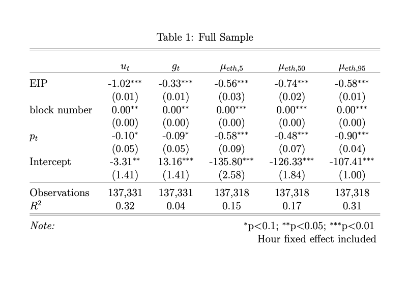
In Table 1, we see that $u_t$ and $g_t$ are negatively related to the ETHUSD rate. We also see that users do indeed take into account the USD value of fees as indicated by the significantly negative coefficients across $\mu_{eth}$ percentiles. In other words, when the ETHUSD rate is high, users lower their bids in ETH. These results imply the coefficient for aggregate fees paid in USD on $p_t$ is .32, .42, and 0 for the 5th, 50th, and 95th percentiles, respectively. The 5th and 10th percentiles are statistically significant, indicating reflexivity, but the 95th percentile is not.
More interestingly, we can split our sample into pre- and post-1559 to see how the results vary. Table 2 shows the results pre-1559 which is the period between block 12,895,000 (7/20/21) and 12,965,000 (8/5/2021).
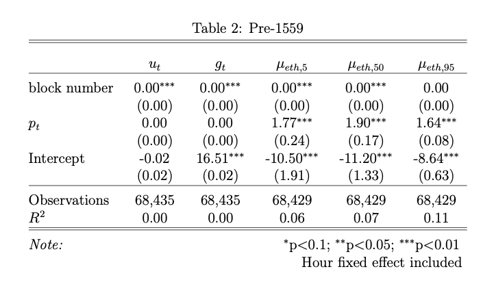
The results for $\mu_{eth}$ pre-1559 are significantly positive and greater than two in USD terms indicating a highly reflexive relationship to the ETHUSD rate. However, in Table 3 we see the results are significantly negative for $\mu_{eth}$ post-1559 between blocks 13,035,000 (8/16/21) and 13,105,000 (8/31/21).
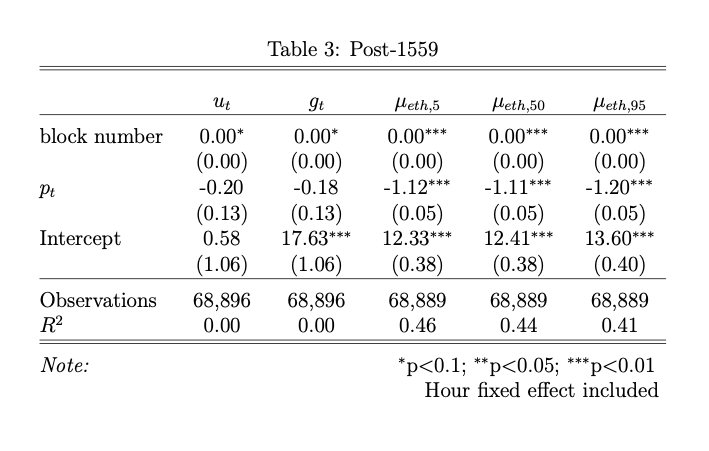
We need to think through the logical reason for this dichotomy more. Arguably, this analysis suffers from omitted variables bias, and I would agree. So, take the results with a grain of salt. However, users adjusting their bids in ETH lower in response to higher ETHUSD rates is consistent with the results of Liu et al. (2022) and Donmez and Karaivanov (2021). We should account for macroeconomic variables and time, since, presumably, they would meaningfully impact our results. With regard to time, we looked at block-level data here, but results may differ when aggregated across different time intervals. Also, take into consideration that we have only observed a month’s worth of data, hardly enough to draw sweeping conclusions. For example, the ETHUSD rate was up 58% during our pre-1559 period and up only 8% post-1559 which may responsible for the large pre-1559 coefficients.
We can quickly apply a different model at a daily frequency including additional variables. Table 4 uses data aggregated at daily intervals where $usd_t$ is the DXY index level, $u_t > .9$ is a binary indicator when network utilization is greater than 90%, EIP is 0 before the introduction of EIP-1559 and 1 afterwards, and BNB is 1 when the ETHUSD price is above the 130-day moving average and 0 otherwise. We can see that $p_t$ and $usd_t$ have negative coefficients whereas high utilization and BNB have positive coefficients, all of which are significant using Newey-West standard errors.
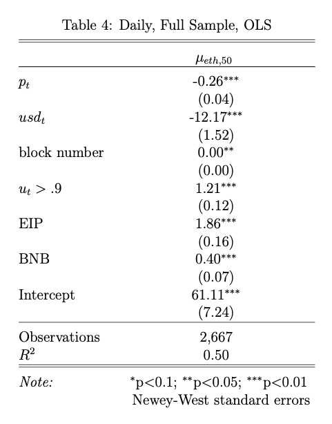
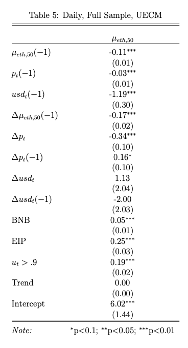
We have been using a standard OLS specification, however, it may be more appropriate to use another model, particularly considering we are interested in potentially nonstationary variables. We may want to use an unconstrained error correction model (UECM). This would allow us to determine the effects of levels and first differences and, thus, long- versus short-term effects. Table 5 shows the results of a UECM with two lags using the variables from Table 4. Our results are similar to the OLS specification but there are additional diagnostic tests we need to run to determine the quality of the model.
Despite the shortcomings mentioned above, the formalization and analysis we have done here is a good starting point for further work.
Seigniorage
In valuation equation $(1)$ seigniorage is $\frac{\theta_tA_t^{$}\pi_t}{1+\pi_t}$. At time $t+1$ the USD value of convenience holdings is equal to:
\[\theta_tA^{\$}_t\bigg(1+\frac{g_{A^{\$}}-\pi_t}{1+\pi_t}\bigg)+s=\theta_tA^{\$}_t(1+g_{A^{$}})\]where $s$ is seigniorage. We assume that convenience holdings are a constant proportion of $A^{$}$, so solving for $s$:
\[\begin{aligned} s &=\theta_tA^{\$}_t(1+g_{A^{$}})-\theta_tA^{\$}_t\bigg(1+\frac{g_{A^{\$}}-\pi_t}{1+\pi_t}\bigg) \\ &= \theta_tA^{\$}_t\bigg[(1+g_{A^{\$}})-\bigg(1+\frac{g_{A^{\$}}-\pi_t}{1+\pi_t}\bigg)\bigg] \\ & = \theta_tA^{\$}_t\bigg[1+g_{A^{\$}}-1-\frac{g_{A^{\$}}-\pi_t}{1+\pi_t}\bigg] \\ &= \theta_tA^{\$}_t\bigg[g_{A^{\$}}-\frac{g_{A^{\$}}-\pi_t}{1+\pi_t}\bigg] \\ &=\theta_tA^{\$}_t\bigg[\frac{g_{A^{\$}}+g_{A^{\$}}\pi_t}{1+\pi_t}-\frac{g_{A^{\$}}-\pi_t}{1+\pi_t}\bigg] \\ &=\theta_tA^{\$}_t\bigg[\frac{(g_{A^{\$}}+g_{A^{\$}}\pi_t)-(g_{A^{\$}}-\pi_t)}{1+\pi_t}\bigg] \\ &=\theta_tA^{\$}_t\bigg[\frac{g_{A^{\$}}+g_{A^{\$}}\pi_t-g_{A^{\$}}+\pi_t}{1+\pi_t}\bigg] \\ &=\theta_tA^{\$}_t\bigg[\frac{g_{A^{\$}}\pi_t+\pi_t}{1+\pi_t}\bigg] \\ &=\theta_tA^{\$}_t\bigg[\frac{\pi_t}{1+\pi_t}\bigg](1+g_{A^{\$}}) \\ &=\frac{\theta_tA^{\$}_t\pi_t}{1+\pi_t}(1+g_{A^{\$}}) \end{aligned}\]The equality of the change in convenience holdings plus an inflation tax:
\[\frac{\theta_tA_t^{\$}\pi}{1+\pi}(1+g_{A^{\$}})=\underbrace{\theta_{}A_{t}^{\$}(1+g_{A^{\$}})-\theta_{t}A_{t}^{\$}}_{\text{change in convenience holdings}}-\underbrace{\frac{g_{A^{\$}}-\pi}{1+\pi}\theta_{t}A_{t}^{\$}}_{\text{inflation tax}}\] \[\begin{aligned} &=\frac{\theta_tA_t^{\$}\pi}{1+\pi}(1+g_{A^{\$}})- (\theta_{t}A_{t}^{\$}(1+g_{A^{\$}})-\theta_{t}A_{t}^{\$})+ \frac{g_{A^{\$}}-\pi}{1+\pi}\theta_{t}A_{t}^{\$} \\ &= \frac{\theta_tA_t^{\$}\pi+\theta_tA_t^{\$}\pi g_{A^{\$}}}{1+\pi}- \theta_{t}A_{t}^{\$}g_{A^{\$}}+ \frac{\theta_{t}A_{t}^{\$}g_{A^{\$}}-\theta_{t}A_{t}^{\$}\pi}{1+\pi}\\ &= \frac{\theta_tA_t^{\$}\pi+\theta_tA_t^{\$}\pi g_{A^{\$}}}{1+\pi} - \frac{\theta_{t}A_{t}^{\$}g_{A^{\$}}+\theta_tA_t^{\$}\pi g_{A^{\$}}}{1+\pi}+ \frac{\theta_{t}A_{t}^{\$}g_{A^{\$}}-\theta_{t}A_{t}^{\$}\pi}{1+\pi}\\ &=0 \end{aligned}\]Issues/Ideas
General
- Cash in advance constraint and a utility function with three goods long-term horizon (1 week, 1 month)
- Note: my model also has $M^\ast$ as a constant multiple of $A$ and the price level is $\frac{1}{p_t}$ where $p_t$ is the ETHUSD rate.
- Potential issue is that we’re assuming utilities are additive. The current model assumes investors go from dollars to ETH which are then staked or lent. Users go from dollars to ETH for consumption.
- Stochastic dynamics
- Liquidity adjusted VaR
- Concept of “value leakage” e.g. accrual of ETH as a derivative of productive ETH activity
- Laffer curve for optimal seigniorage
- Choice of whether to delegate, create a pool, or solo stake source
- What happens if stETH becomes numeraire?
- Disproportionate impact of validator queue on pools of different sizes
- Borrow rates for stETH relative to ETH?
- Be clear about observables and unobservables
- Any risk averse staker will prefer pooled staking (not including fees)
Issuance
- Need to add variance of MEV
- Variance as a function of the percentage staked
- Clean up staker optimization problem, make it solveable
- Currently risky to run single validator from one node given slashing risk here
- Verify: experience shows that correlated slashes is not a single event and tend to be spread over time, where you can have time to react to stop the bleeding.
- It’s easier to mitigate large slashing events, i.e. script that shuts down all validators if one get slashed.
- Node creation non-zero cost, costless for new validator from single node
- Just set range to be [min, 2 x min] to neutralize size yield differentials
- Can I add to the EB of my validator? If so, in what increments?
ETH/stETH rate
- Account for slashing risk, rewards, and potential convenience for leverage
- Risk is much a higher for a solo staker than liquid staking protocol?
- What is $T$ with different preferences for using buffer inflows and staking directly from Ethereum?
- Clarify: Instant liquidity needed right now.
Objective function
- Need to formalize the profit to attack
- Parse censorship resistance and trustlessness
- Does not explicitly consider stake pool operators that personally do not have any, or a relatively small percentage of, ETH staked.
- Equation $(45)$ captures their ability to collude but we need to formalize what is at stake for such a stake pool operator. The entity can try to (a) steal the pooled ETH (b) attack the network, including censoring transactions, or (c) earn the present discounted value of future cash flows from pool operations.
- Censorship-resistance as a strong-form of liveness
- Issue is with the Nakamoto Coefficient. If we added pools to the dimensions, Lido would make $\hat{\Phi}$ equal to 1. However, this does not discriminate between types of pools that can be considered more, or less, risky to Ethereum. Ideally, we would like the minimum number of entities that need to be compromised based on their risk-adjusted similarity, e.g. if two entities have the exact same risk-adjusted characteristics then they are practically one entity. The risk-adjustment, while subjective, would allow us to adjust the weight of being a part of Lido lower relative to some other protocol that is deemed riskier, e.g. one that censors.
- We would also like to keep the intuitiveness of the Nakamoto coefficient.
- Consider the cost to censor transactions. The amount of time it takes for a transaction to be included in a block as a function of the total transaction fee? The amount foregone is equal to $kT$ where $k$ is the number of blocks and $T$ is the total amount in censored tips in the uncongested case. In the congested case it’s $T-L$ where $L$ is the smallest tip (plus MEV) in the list of included transactions. The minimum amount an adversary would have to bribe a block proposer to censor.
- How many blocks it takes a certain transaction that is willing to pay more than or equal to the minimum amount paid (base + tip) in the block in the congested case and base in the uncongested case to be included. Entities can attempt to perform any of the three of a, b, and c above individually or pair (a) with (b) or (b) with (c). The risks of (a) and (b) to the protocol are still captured by $(45)$. Perhaps this says something about the functional form of $(42)$ which might be $\Psi_t^{\hat{\Phi}_t}$. Slashing or censoring transactions is “risky” because it reduces (c).
- See Resnick, Pai, and Fox (2023)
Investor objective function
- Is the risk not getting dollars or ETH?
- Inability to rebalance both ETH and broader portfolio
- Simply, the difference between the initial value of the portfolio and post-liquidation value.
- Ignoring buffers, the liquidation return to illiquid staking should equal the discount on the liquid staking token?
- What would make someone indifferent between liquidating in X days and liquidating today at a discount?
- So, would illiquid just be $\frac{1}{S^y(1+i)^T}$?
- With the buffer, this would mean that the price on a liquid staking token is always greater than or equal to the illiquid staking option.
- Convenience yield for ease of leverage?
- So, would illiquid just be $\frac{1}{S^y(1+i)^T}$?
- What’s the fundamental difference between validator A collateralizing their staked ETH via some off-chain agreement and validator B, who is the exact same as A except they have a digital representation of a claim to their stake?
- What would make someone indifferent between liquidating in X days and liquidating today at a discount?
- Ignoring buffers, the liquidation return to illiquid staking should equal the discount on the liquid staking token?
- Assume once withdrawn from any of the three assets, you just have to wait.
- It’s just more convenient to have the liquid staking token (?)
- Let’s assume away solo staking and just say those people have some different objective function
- Then it’s between liquid staking solutions
- Let’s assume they’re all structured the same way and thus priced the same way
- Then it’s between liquid staking solutions
- Consider optimal liquidation strategies, there’s a certain amount able to be withdrawn immediately, then the choice is to sell the staked or lent derivative at a discount or wait in the exit queue, the same as a solo staker. Perhaps think about integrating the staked derivative price itself since it reflects all of this?
- Alternatively, and perhaps more simply, following Lo, Petrov, and Wierzbicki (2003) we can express it as:
where $\theta$ determines the weight placed on liquidity and $\ell$ is a vector of liquidity metrics for solo staking, lending and various liquid staking protocols cross-sectionally normalized between 0 and 1. There are two types of liquidity: redemption and liquid token. We can take an average of the normalized liquidity metrics to create $\ell$.